MATHEMATICAL MODEL OF EVAPORITE VOID EVOLUTION (EVE)
Outline of modelling approach
The translation of the conceptual model into its mathematical equivalent is based on the karst simulation model CAVE (Carbonate Aquifer Void Evolution), which has recently been developed by UTAG with EC Framework III funding. The basic features of CAVE are briefly summarised below. More details are given by Clemens et al. (1996), Younger et al. (1997) and Hückinghaus et al. (1999).
A karst aquifer may be conceptualised as a flow system consisting of a so-called fissured system, which represents the mass of the fractured rock, and a conduit system representing the karst tube network. Groundwater flow in the fissured system is modelled using the Boussinesq equation (e. g. Berkowitz et al. 1988). Flow in the conduit system is governed by Kirchhoff's law, stating that total inflow and total outflow are in balance for each node of the conduit network (Horlacher & Lüdecke, 1992). For each tube the discharge is related to the head difference by the Darcy-Weisbach equation which is appropriate for both laminar and turbulent flow conditions. Exchange of groundwater between the conduits and the fissured system is assumed to be proportional to the hydraulic head difference between these flow domains (Sauter, 1992).
In order to simulate the evolution of voids, the flow model is coupled to a limestone dissolution module, which calculates the dissolution rates in circular tubes. For the purposes of ROSES, the limestone dissolution module of CAVE has been replaced by an evaporite dissolution module, which yielded a new simulation tool named EVE. The first step in the development of EVE was to assess the dissolution kinetics of gypsum.
Assessment of gypsum dissolution kinetics
Gypsum dissolution is composed of two steps: firstly, a heterogeneous reaction at the mineral surface, and secondly the diffusion of the dissolved molecules across a thin diffusion boundary layer into the bulk solution.
The surface reaction rate Rsurf depends on the reaction rate constant k, the equilibrium concentration ceq, the surface concentration csurf and the reaction order n:
![]() (1)
(1)
The diffusion rate Rdiff depends on the mass transfer coefficient h (which is a function of the diffusion coefficient D and the thickness of the diffusion boundary layer d ), the surface concentration csurf and the concentration in the bulk solution c:
![]() (2)
(2)
Most experiments indicate that the surface reaction is very fast compared to the rate of diffusion across the boundary layer (e. g. Liu & Nancollas, 1970; Barton & Wilde, 1971; James & Lupton, 1978; Liu & Dreybrodt, 1997). This would imply that the surface concentration equals the equilibrium concentration. Dissolution of gypsum then obeys a first-order rate law, wherein th rate constant is only a function of the diffusion coefficient and the thickness of the boundary layer:
![]() (3)
(3)
The mixed transport/reaction control of gypsum proposed by Raines & Dewers (1997) holds that the dissolution rate constant would, in addition, depend on the surface reaction rate constant. The basis of this proposal has been questioned by Dreybrodt & Gabrovšek (1998) who concluded that ‘the experimental data and their interpretation given by Raines and Dewers cannot be regarded as sufficiently reliable to draw conclusions on the surface reaction rate laws of gypsum’. This consideration of dissolution kinetics has concluded that gypsum dissolution is entirely controlled by the diffusion across the boundary layer and, for the purposes of the EVE code development, can be described by equation (3).
Implementation of gypsum dissolution kinetics in EVE
Since the diffusion coefficients of Ca2+ and SO42- are known (e. g. Dreybrodt 1988), only the thickness of the diffusion boundary layer has to be determined to obtain the dissolution rate constant. The dimensionless ratio of tube diameter and boundary layer thickness is called the Sherwood number:
![]() (4)
(4)
Where d = tube diameter, d = boundary layer thickness, and D = diffusion coefficient. The Sherwood number expresses the relationship between advective and diffusive mass transport and basically determines the saturation length, i. e. the distance after which saturation has been achieved.
Due to the slow diffusive mass transfer of Ca2+ and SO42- the uniform concentration of water entering a tube cannot be replaced instantaneously with higher concentrations resulting from gypsum dissolution at the the tube wall. Therefore, a diffusion boundary layer develops along the surface of the tube. The boundary layer is fully developed, when it reaches the centre of the tube. Therefore, far from the tube entrance, the Sherwood number is a constant i.e. 3.66 for laminar flow conditions in a circular tube (Beek & Muttzall 1975). The dissolution rate constant is simply a function of tube diameter and diffusion coefficient:
![]() (5)
(5)
However, near the tube entrance, the thickness of the boundary layer also depends on the distance from the entrance and on the flow velocity. So far only the case far from a tube entrance has been implemented in EVE. Further code development will decide whether this approach is sufficient for the conceptual settings to be modelled within the ROSES project or if tube length and flow velocity have to be taken into consideration.
Modelling of conceptual settings
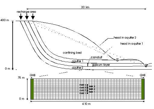
In order to test the EVE code, the simplest conceptual situation described in section 2.1 was chosen; i.e. a single conduit in a gypsum layer sandwiched between two confined aquifers. Instead of modelling the whole regional system, flow was simulated only in a small section. Simulations used a general head boundary condition, i. e. the flow across the boundaries is calculated from the head difference between the boundary cells and the recharge and discharge area, respectively. The model is constructed such that the recharge area is 10 km to the left of the model centre and discharge areas are at 5 km (aquifer 1) and 10 km (aquifer 2) to the right of the model centre.
The cross-section is a slice of 10 m width. This value can be interpreted as the distance between the conduits perpendicular to the cross-section. The hydraulic conductivity is assumed to be 10-6 m/s for the aquifers and 10-9 m/s for the gypsum layer. Each layer has a thickness of 25 m. The conduit is subdivided into three tubes, and an exchange of water between the conduit and the fissured system is allowed at the four nodes. The concentration of Ca2+ and SO42- water flowing in the aquifers is assumed zero, whilst the water from the gypsum layer is saturated with respect to gypsum (15.4 mmol/l according to Liu & Dreybrodt 1997). Because the hydraulic head in the lower aquifer is higher than in the upper aquifer, the flow is directed upwards
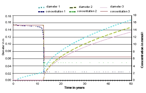
To start with, only tube 1 is enlarged. The second and the third tube remain at a small diameter for more than ten years, and prevent any increase in the discharge through the conduit. This situation corresponds to the early stages of speleogenesis, when discharge is dependent on the hydraulic conductivity of the conduit (internal hydraulic control). At this stage water entering the first tube with concentration zero is almost saturated at the outlet of tube 1. The dissolution process stops within the second tube, because the water becomes fully saturated. A noticeable enlargement of the second tube is only possible if the concentration at the outlet of the first tube decreases significantly. The breakthrough, which is characterized by a considerable enlargement of the tubes accompanied by an increase in discharge and a decrease in concentration, occurs after twelve years. From then on the concentrations at the outlets of the tubes remain constant, far below saturation. The tubes reach diameters of 130 to 170 mm after 50 years. This late stage is the main stage of artesian speleogenesis with an external hydraulic control. The discharge is now controlled by the boundary conditions and the hydraulic conductivity of the aquifers, but not by the diameter of the conduit.
Due to the enlargement of the tubes, the hydraulic heads in the conduit system vary with time. Initially, the head difference between each pair of nodes is about 4 m. When the first tube has reached a certain diameter, the head difference between nodes 1 and 2 becomes zero and the head difference along the other tubes increases accordingly. Once the second tube has reached a certain diameter, the total head difference of about 12 m is along the third tube. This causes an increase in the discharge through the conduit. Since the water within the third tube is now below saturation, the interaction between concentration and discharge causes a very fast breakthrough. The increase in the flow rate implies an enlargement of the tube and vice versa. These first modelling results show that EVE is capable of simulating the basic features of the scenario studied here. Therefore, it appears to be justified to assume that reliable model results will be produced when further scenarios are investigated.
|